Um punhado de Monads
Quando nós começamos a falar sobre functors, vimos que elas foram conceitos úteis para os valores que poderiam ser mapeados. Então, nós tornamos esse conceito um passo a mais atrávez da introdução da applicative functors, o que nos permite ver certos tipos de valores como valores com contexto e utilizar funções normais nesses valores enquanto preserva-se o significado desses conceitos.
Neste capítulo, nós vamos estudar sobre monads, que apenas reforça applicative functors. Muito semelhante a applicative functors que somente reforça functors.

Quando nós começamos com functors, vimos que é possível mapear funções de vários tipos de dados. Nós vimos que para esse propósito, o tipo de classe Functor nos foi apresentado o que nos levou a fazer a seguinte pergunta: quando temos um tipo de função a -> b e também um tipo de dado f a, como nós fazemos para mapear essa função para terminar com um tipo de dado f b? Nós vimos como mapear somente um Maybe a, uma lista [a], um IO a etc. Nós até vimos como mapear uma função a -> b para outra função do tipo r -> a para obter uma função do tipo r -> b. Para responder essa pergunta de como mapear uma função para algum tipo de dado, tudo o que nós temos que fazer é olhar para o tipo de dado fmap:
fmap :: (Functor f) => (a -> b) -> f a -> f b
E então fizemos funcionar para nossos tipos de dados escrevendo instâncias apropriadas de Functor.
Em seguida vimos uma possibilidade de melhorar as functors e dizer, ei, e se essa função a -> b já estiver empacotada dentro de um functor value? Por exemplo, e se nós tivermos Just (*3), como nós fazemos para aplicar isso a Just 5? E se nós não quisermos aplicar para Just 5 mas em vez disso para um Nothing? Ou se nós temos [(*2),(+4)] como podemos aplicar isso a [1,2,3]? Como isso funciona mesmo? Por isso, o tipo de classe Applicative foi introduzido, no qual queremos a resposta para o seguinte tipo:
(<*>) :: (Applicative f) => f (a -> b) -> f a -> f b
Vimos também que podemos ter um valor normal e empacota-lo dentro de um tipo de dado. Por exemplo, podemos ter 1 e empacota-lo de modo a se tornar um Just 1. Ou podemos transforma-lo em [1]. Ou em uma ação de I/O que não faz nada e apenas produz 1. A função que faz isso é chamada de pure.
Como dissemos, um valor de aplicativo pode ser visto como um valor com um contexto adicional. Um valor imaginário, incluído em termos técnicos. Por exemplo, o caractere 'a' é apenas um caractere normal, enquanto que Just 'a' tem algum contexto adicionado. Em vez de um Char, nós temos um Maybe Char, que nos diz que o valor pode ser um caractere, mas também pode ser uma ausência de um caractere.
Foi ótimo ver como o tipo de classe Applicative nos permitiu usar funções normais nesses valores com contexto e como que o contexto foi preservado. Observe:
ghci> (*) <$> Just 2 <*> Just 8
Just 16
ghci> (++) <$> Just "klingon" <*> Nothing
Nothing
ghci> (-) <$> [3,4] <*> [1,2,3]
[2,1,0,3,2,1]
Ah, legal, agora que tratamos eles como valores de aplicativo, Maybe a representa valores calculados que podem ter falhado, [a] representa valores calculados que tem vários resultados (cálculos não determinísticos), IO a são valores que representam valores que tem efeitos colaterais, etc.
Monads são extensões naturais de applicative functors e com elas estamos preocupados com isto: Se você tem um valor com um contexto, m a, como você aplica isto a uma função que tem um contexto normal a e retorna um valor com um contexto? Quer dizer, como você aplica uma função do tipo a -> m b para um valor do tipo m a? Assim, basicamente nós vamos querer essa função:
(>>=) :: (Monad m) => m a -> (a -> m b) -> m b
Se você tem um valor imaginário e uma função que tem um valor normal mas retorna um valor imaginário, como fazemos para alimentar este valor imaginário em uma função? Esta é a principal questão que vamos nos preocupar quando estivermos lidando com monads. Nós escrevemos m a em vez de f a porque o m significa Monad, mas monads são apenas applicative functors que suportam >>=. A função >>= é pronunciada como bind.
Quando nós temos um valor normal a e uma função normal a -> b é realmente fácil alimentar o valor da função - você apenas aplica a função com o valor que vem com determinado contexto, é preciso um pouco de pensamento para ver como esses valores imaginários são alimentados em funções e como levam em conta o seu comportamento, mas você vai ver como é fácil como um, dois três.
Molhando os pés com Maybe

Agora que nós temos uma vaga ideia sobre o que são monads, vamos ver se podemos tornar essa ideia um pouco menos vaga.
Para a grande surpresa de ninguém, Maybe é um monad, então vamos explora-lo um pouco mais e ver se podemos combina-lo com o que nós aprendemos sobre monads.
Um valor do tipo Maybe a representa um valor do tipo a com o contexto de uma possível falha anexada. Um valor de Just "dharma" significa que a string "dharma" existe enquanto que o valor de Nothing representa sua ausência, ou se você olhar para a string como um resultado de um cálculo, isso significa que o cálculo falhou.
Quando nós olhamos para Maybe como uma functor, vimos que se iterarmos uma função fmap sobre ela, ela será mapeada internamente se o valor for Just, caso contrário o Nothing será mantido porque não há nada para mapear.
Assim:
ghci> fmap (++"!") (Just "wisdom")
Just "wisdom!"
ghci> fmap (++"!") Nothing
Nothing
Assim como um applicative functor, que funciona de forma semelhante. Contudo, applicatives também tem a função de embalar as coisas. Maybe é um applicative functor de tal forma que, quando usamos <*> para aplicar uma função dentro de um Maybe para um valor que está dentro de um Maybe, ambos tem que ser Just para o resultado ser um valor Just, caso contrário o resultado é Nothing. Faz sentido porque se você tiver perdido a função ou a coisa que você está aplicando, você não poderá fazer nada lá fora com o ar rarefeito, então você terá que propagar uma falha:
ghci> Just (+3) <*> Just 3
Just 6
ghci> Nothing <*> Just "greed"
Nothing
ghci> Just ord <*> Nothing
Nothing
Quando usamos o estilo applicative para ter funções normais agindo em valores Maybe isto é semelhante. Todos os valores têm que ser Just, caso contrário todos são Nothing!
ghci> max <$> Just 3 <*> Just 6
Just 6
ghci> max <$> Just 3 <*> Nothing
Nothing
E agora vamos pensar como faríamos >>= para Maybe. Como nós falamos, >>= tem um valor monadico, e uma função que tem um valor normal e retorna um valor monadico e consegue aplicar essa função para um valor monadico. Como ele faz isso, se a função tem um valor normal? Bem, para fazer isso, ele tem que levar em conta o contexto desse valor monadico.
Neste caso, >>= levaria um valor Maybe a e uma função do tipo a -> Maybe b que de alguma maneira aplica a função para o Maybe a. Para descobrir como ele faz isso, podemos usar a intuição que temos de Maybe ser um applicative functor. Digamos que temos uma função \x -> Just (x+1). Ela pega um número, acrescenta 1 a ele e o embala com um Just:
ghci> (\x -> Just (x+1)) 1
Just 2
ghci> (\x -> Just (x+1)) 100
Just 101
Se alimentarmos ela com 1, ela será calculada como Just 2. Se nós dermos a ela o número 100, o resultado será Just 101. Muito simples. Agora aqui vai o chute: Como nós alimentamos um valor Maybe para esta função? Se nós pensarmos sobre como Maybe atua como um applicative functor, responder isso será muito fácil. Se alimentarmos isso com um valor Just, pegarmos o que está dentro de Just e aplicarmos a função nele. Se der a ele um Nothing, hmm, bem, então estaremos com uma função porém Nothing (nada) para aplicar nela. Neste caso vamos apenas fazer o que nós fizemos antes de dizer que o resultado é Nothing.
Ao invés de chamar isso de >>=, iremos chama-lo de applyMaybe por enquanto. Ela irá pegar um Maybe a e uma função que retorna um Maybe b e manipula-los para aplicar esta função ao Maybe a. Aqui está o código:
applyMaybe :: Maybe a -> (a -> Maybe b) -> Maybe b
applyMaybe Nothing f  = Nothing
applyMaybe (Just x) f = f x
Ok, agora vamos jogar com ele um pouco. Vamos usa-lo como uma função infixa com o valor de Maybe no lado esquerdo e a função no lado direto:
ghci> Just 3 `applyMaybe` \x -> Just (x+1)
Just 4
ghci> Just "smile" `applyMaybe` \x -> Just (x ++ " :)")
Just "smile :)"
ghci> Nothing `applyMaybe` \x -> Just (x+1)
Nothing
ghci> Nothing `applyMaybe` \x -> Just (x ++ " :)")
Nothing
No exemplo acima, nós vimos que quando usamos applyMaybe com um valor Just e uma função, a função simplesmente será aplicada no valor dentro de Just. Quando tentarmos usar isso com um Nothing, o resultado completo será Nothing. Que tal se a função retornar apenas um Nothing? Vamos ver:
ghci> Just 3 `applyMaybe` \x -> if x > 2 then Just x else Nothing
Just 3
ghci> Just 1 `applyMaybe` \x -> if x > 2 then Just x else Nothing
Nothing
Exatamente o que nós esperávamos. Se o valor monadico à esquerda é um Nothing, a coisa toda é Nothing. E se a função a direita retorna um Nothing, o resultado novamente é Nothing. Isto é muito similar quando nós usamos Maybe como um applicative e nós obtemos um resultado Nothing se em alguma parte havia um Nothing.
Parece que para Maybe, nós temos que descobrir como tiramos um valor imaginário e alimentamos ele com uma função que recebe um valor normal e retorna um imaginário. Nós fazemos isso mantendo em mente que um valor Maybe representa um cálculo que pode ter falhado.
Você pode estar se perguntado, como é que isso pode ser útil? Pode parecer que applicative functors são mais fortes que monads, quando applicative functors nos permitem ter uma função normal para faze-la funcionar operando em valores com contextos. Vamos ver que monads podem fazer isso também, porque eles são uma evolução de applicative functors, e que eles também podem fazer alguma coisas legais que applicative functors não podem.
Iremos voltar para Maybe em um minuto, mas primeiro, vamos verificar que tipo de classe pertence a monads.
O tipo de classe Monad
Assim como functors tem o tipo de classe Functor e applicative functors tem o tipo de classe Applicative, monads tem seu próprio tipo de classe: Monad! Wow, quem teria adivinhado? Assim é como esse tipo de classe se parece:
class Monad m where
    return :: a -> m a

    (>>=) :: m a -> (a -> m b) -> m b

    (>>) :: m a -> m b -> m b
    x >> y = x >>= \_ -> y

    fail :: String -> m a
    fail msg = error msg

Vamos começar com a primeira linha. Ela diz: class Monad m where. Mas espere, nós não dizemos que monads são apenas reforços de applicative functors? Não deveria haver uma restrição de classe ao longo das linhas de class (Applicative m) = > Monad m where devendo assim o tipo ser primeiro um applicative functor antes de produzir um monad? Bem, não deveria, mas quando Haskell foi criado, não tinha ocorrido ser uma boa opção para Haskell. Mas com certeza, cada monad é um applicative functor, mesmo se a declaração não dizer isso.
A primeira função que o tipo de classe Monad define é return. É o mesmo que pure, somente com um nome diferente. Esse tipo é (Monad m) => a -> m a. É preciso um valor para colocá-lo em um contexto padrão mínimo que ainda mantém esse valor. Em outras palavras, é preciso alguma coisa para envolver ele em um monad. Ele sempre faz a mesma coisa com a função pure para o tipo de classe Applicative, o que significa que já estamos familiarizados com return. Nós já usamos return quando fizemos I/O. Usamos ele para pegar um valor e fazer uma ação fictícia de I/O que não faz nada mas que produz um valor. Para Maybe ele cria um valor e envolve ele em um Just.

A próxima função é >>=, ou bind. É como um function application, só que em vez de ter um valor normal e alimentar ele para uma função normal, ele tem um valor monadico (ou seja, um valor com um contexto) e alimenta ele para uma função que recebe um valor normal, mas retorna um valor monadico.
Em seguida, temos >>. Nós não vamos prestar muita atenção nisso agora porque ele vem com uma implementação padrão e nós praticamente nunca implementamos isso ao criar instâncias de monads.
A última função do tipo de classe Monad é fail. Nós nunca usamos ela explicitamente em nosso código. Em vez disso, ela é usada pelo Haskell para permitir falhas em um construtor semântico especial para monads que iremos conhecer depois. Nós não precisamos nos preocupar com fail por hora.
Agora que nós sabemos como que o tipo de classe Monad se parece, vamos dar uma olhada em como Maybe é uma instância de Monad!
instance Monad Maybe where
    return x = Just x
    Nothing >>= f = Nothing
    Just x >>= f  = f x
    fail _ = Nothing
return é o mesmo que pure, assim não nos exige esforços. Nós fazemos o mesmo que fizemos no tipo de classe Applicative e envolvemos ele em um Just.
A função >>= é o mesmo que o nosso applyMaybe. Quando alimentamos o Maybe a para nossa função, nós temos em mente o contexto e retornamos um Nothing se o valor da esquerda é Nothing porque se não há nenhum valor, então não há nenhuma maneira de aplicar a nossa função nele. Se é um Just pegamos o que está dentro da função e aplicamos f.
Nós podemos brincar por ai com Maybe como sendo um monad:
ghci> return "WHAT" :: Maybe String
Just "WHAT"
ghci> Just 9 >>= \x -> return (x*10)
Just 90
ghci> Nothing >>= \x -> return (x*10)
Nothing
Nada de novo ou emocionante na primeira linha uma vez que já usamos pure com Maybe e nós sabemos que return é apenas pure com um nome diferente. As próximas duas linhas >>= mostram um pouco mais.
Note que quando nós oferecemos Just 9 para a função \x -> return (x*10), o x assumiu o valor 9 dentro da função. Parece que fomos capazes de extrair o valor de Maybe sem pattern-matching. E nós ainda não perdemos o contexto do nosso valor Maybe, porque quando ele é Nothing, o resultado do uso >>= vai ser Nothing também.
Ande na linha
Agora que sabemos como alimentar um valor Maybe a para uma função do tipo a -> Maybe b, tendo em vista o contexto de uma possível falha, vamos ver como podemos usar >>= várias vezes para lidar com cálculos de vários valores de Maybe a.
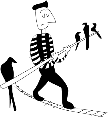
Pierre decidiu fazer uma pausa em seu trabalho na fazenda de peixes e tentar caminhar em uma corda banda. Isso não é ruim para ele, mas ele tem um problema: pássaros mantem seu pouso em ponto de equilíbrio! Eles vêm e descansam um pouco, batem um papo com seus amigos pássaros e depois decolam a procura de migalhas de pão. Isso não incomodaria tanto ele se o número de aves no lado esquerdo do bastão fosse sempre igual ao número de aves no lado direito. Mas às vezes, todos os pássaros decidem que eles gostam de um lado e assim ele desequilibra-se, o resultado é uma queda embaraçosa para Pierre (ele está usando uma rede de segurança).
Digamos que ele mantém o seu equilíbrio, se a diferença do número de pássaros do lado esquerdo do bastão em relação ao número de pássaros do lado direito seja três. Assim, se tem um passado do lado direito e quatro pássaros do lado esquerdo, ele está em equilibrio, Mas se um quinto pássaro pousa no lado esquerdo, ele perde o equilíbrio e leva um tombo.
Vamos simular pássaros pousando e voando longe do bastão e ver se Pierre ainda está nele depois de um determinado número de pássaros chegando e partindo. Por exemplo, queremos ver o que acontece com Pierre se o primeiro pássaro chega no lado esquerdo, em seguida, quatro pássaros ocupam o lado direito e depois o pássaro que estava no lado esquerdo decide voar para longe.
Podemos representar o bastão com um simples par de números inteiros. O primeiro componente irá significar o número de aves no lado esquerdo e o segundo componente o número de aves no lado direito:
type Birds = Int
type Pole = (Birds,Birds)
Primeiro criamos um tipo sinônimo para Int, chamados de Birds, porque estamos usando números inteiros para representar quantos pássaros existem. Em seguida criamos um tipo sinônimo de (Birds,Birds) e chamamos ele de Pole (para não ser confundido com uma pessoa de ascendência polonesa).
Em seguida, que tal criar uma função que recebe um número de pássaros e pousa eles em um lado do bastão. Aqui estão as funções:
landLeft :: Birds -> Pole -> Pole
landLeft n (left,right) = (left + n,right)

landRight :: Birds -> Pole -> Pole
landRight n (left,right) = (left,right + n)
Coisa muito simples. Vamos testa-los:
ghci> landLeft 2 (0,0)
(2,0)
ghci> landRight 1 (1,2)
(1,3)
ghci> landRight (-1) (1,2)
(1,1)
Para fazer os pássaros voarem para longe nós apenas recebemos um número negativo de pássaros pousando em um lado. Porque pousar um pássaro em Pole retona um Pole, podemos encadear a aplicação de landLeft e landRight:
ghci> landLeft 2 (landRight 1 (landLeft 1 (0,0)))
(3,1)
Quando aplicamos a função landLeft 1 para (0,0) temos (1,0). Então, pousamos um pássaro no lado direito, resultando em (1,1). Finalmente dois pássaros pousam no lado esquerdo, resultando em (3,1). Nós aplicamos uma função em algo escrevendo primeiro a função e depois escrevendo os parâmetros, mas aqui será melhor se o bastão vier primeiro e depois a função de pouso. Se fizermos uma função assim:
x -: f = f x
Podemos aplicar funções escrevendo primeiro os parâmetros e depois a função:
ghci> 100 -: (*3)
300
ghci> True -: not
False
ghci> (0,0) -: landLeft 2
(2,0)
Ao usar isso, podemos repetidamente pousar pássaros no bastão de um modo mais legível:
ghci> (0,0) -: landLeft 1 -: landRight 1 -: landLeft 2
(3,1)
Muito legal! Este exemplo é equivalente ao anterior, onde repetidamente pousamos os pássaros no bastão, porém ele é mais legível. Aqui, está mais obvio que começamos com (0,0) e depois pousamos um pássaro na esquerda, depois outro na direita e finalmente dois na esquerda.
Até agora está bom, mas o que acontece se 10 pássaros pousam em um lado?
ghci> landLeft 10 (0,3)
(10,3)
10 pássaros no lado esquerdo e somente 3 no lado direito? Isso com certeza vai fazer o pobre Pierre cair no ar! Isso é bastante obvio aqui, mas o que acontece se tivermos uma sequência de pousos assim:
ghci> (0,0) -: landLeft 1 -: landRight 4 -: landLeft (-1) -: landRight (-2)
(0,2)
Podemos pensar que está tudo certo, mas se você seguiu os passos até aqui, vai vai notar que no momento existem 4 pássaros no lado direito e nenhum pássaro no lado esquerdo! Para corrigir isso, precisamos dar mais uma olhada em nossas funções landLeft e landRight. Pelo que percebemos, queremos que essas funções possam falhar. Ou seja, queremos que elas retornem um novo bastão se o equilíbrio estiver certo, mas que falhem se os pássaros pousarem de forma desequilibrada. E qual a melhor maneira de adicionar um contexto de falha a um valor do que usar Maybe! Vamos refazer essa função:
landLeft :: Birds -> Pole -> Maybe Pole
landLeft n (left,right)
    | abs ((left + n) - right) < 4 = Just (left + n, right)
    | otherwise                    = Nothing

landRight :: Birds -> Pole -> Maybe Pole
landRight n (left,right)
    | abs (left - (right + n)) < 4 = Just (left, right + n)
    | otherwise                    = Nothing
Em vez de retornar um Pole esta função agora retorna um Maybe Pole. Ela ainda tem o número de pássaros do antigo bastão como antes, mas em seguida ela verifica se o pouso de muitos pássaros no bastão deixaria Pierre em desequilíbrio. Usamos guardas para verificar se a diferença entre o número de pássaros e o novo bastão é menor do que 4. Se for, evolvemos o novo bastão em um Just e retornamos ele. Se não for, retornamos um Nothing, indicando uma falha.
Vamos ver esses bebês de uma vez:
ghci> landLeft 2 (0,0)
Just (2,0)
ghci> landLeft 10 (0,3)
Nothing
Legal! Quando pousamos pássaros sem deixar Pierre em desequilíbrio, recebemos um novo bastão envolvido em um Just. Mas quando vários pássaros ficaram em um só lado do bastão, recebemos um Nothing. Isso é legal, mas parece que perdemos a habilidade de repetidamente pousar pássaros no bastão. Nós não podemos mais fazer landLeft 1 (landRight 1 (0,0)) porque quando aplicamos landRight 1 para (0,0), nós não recebemos mais um Pole, mas um Maybe Pole. landLeft 1 pega um Pole e não um Maybe Pole.
Precisamos de uma maneira de ter um Maybe Pole e alimentar isso para uma função que leva um Pole e retorna um Maybe Pole. Felizmente, temos >>=, que faz exatamente isso para Maybe. Vamos dar uma olhada:
ghci> landRight 1 (0,0) >>= landLeft 2
Just (2,1)
Lembre-se, landLeft 2 tem um tipo de Pole -> Maybe Pole. Não poderíamos simplesmente alimentar este Maybe Pole que é o resultado de landRight 1 (0,0), assim nós usamos >>= para receber esse valor com um contexto e devolvê-lo a landLeft 2. >>= de fato nos permite tratar o valor de Maybe como um valor com um contexto porque se jogarmos um Nothing para dentro de landLeft 2, o resultado será Nothing e uma falha será propagada:
ghci> Nothing >>= landLeft 2
Nothing
Com isso, podemos agora encadear pousos que podem falhar porque >>= nos permite alimentar um valor monadico para uma função que leva um valor normal.
Aqui está a sequência dos pássaros pousando:
ghci> return (0,0) >>= landRight 2 >>= landLeft 2 >>= landRight 2
Just (2,4)
No início, usamos return para pegar um bastão e envolver ele em um Just. Poderíamos simplesmente ter aplicado landRight 2 para (0,0), isso seria o mesmo, mas desta forma podemos ser mais consistentes utilizando >>= para todas as funções. Just (0,0) é alimentado para landRight 2, resultando em Just (0,2). Que, por sua vez, é alimentado para landLeft 2, resultando em Just (2,2), e assim por diante.
Lembre-se, no exemplo de antes introduzimos falha dentro da rotina de Pierre:
ghci> (0,0) -: landLeft 1 -: landRight 4 -: landLeft (-1) -: landRight (-2)
(0,2)
Isso não simula muito bem sua interação com os pássaros, porque no meio há um desequilíbrio, mas o resultado não reflete isso. Mas vamos ver agora como usamos aplicações monadic (>>=) ao invés de aplicações normais:
ghci> return (0,0) >>= landLeft 1 >>= landRight 4 >>= landLeft (-1) >>= landRight (-2)
Nothing

Incrível. O resultado final representa uma falha, que é exatamente o que esperávamos. Vamos ver como esse resultado foi obtido. Primeiro, return envia (0,0)para o contexto padrão, tornando isso um Just (0,0). Em seguida, ocorre o Just (0,0) >>= landLeft 1 . Uma vez que o Just (0,0) é um valor Just, landLeft 1 é aplicado para (0,0), resultando em um Just (1,0), porque os pássaros ainda estão relativamente em equilíbrio. Em seguida, Just (1,0) >>= landRight 4 toma lugar e resulta em Just (1,4) com o equilíbrio dos pássaros ainda intacto, embora somente um pouco. Just (1,4) é enviado para landLeft (-1). Isso significa que landLeft (-1) (1,4) toma o lugar. Por causa da forma como landLeft funciona, isso resulta em um Nothing, porque o bastão resultante esta fora de equilíbrio. Agora que temos um Nothing, ele é enviado para landRight (-2), mas como isso é um Nothing, o resultado é automaticamente Nothing, já que não temos nada para aplicar em landRight (-2).
Nós não poderíamos ter conseguido isso apenas usando Maybe como um applicative. Se você tentar isso, você vai ficar preso, porque applicative functors não permitem que os applicative values interajam muito bem uns com os outros. Eles podem, quando muito, ser usados como parâmetros em uma função usando o estilo applicative. Os operadores de aplicativos vão buscar esses resultados a alimentá-los para a função de maneira apropriada para cada aplicativo, e depois, colocar o valor do aplicativo final junto, mas não são muito interativos entre si. Aqui, porém, cada passo é baseado no resultado anterior. Em cada pouso, o possível resultado anterior é examinado e o bastão é marcado como equilibrado. Isso determina se o pouso vai ter sucesso ou falha.
Nós podemos também inventar uma função que ignora o número atual de pássaros em equilíbrio no bastão apenas fazendo Pierre desequilibrar e cair. Podemos chamar isso de banana:
banana :: Pole -> Maybe Pole
banana _ = Nothing
Agora podemos encadear isso junto com nossos pássaros pousando. Ele sempre fará nosso caminho falhar, porque ignora o que esta recebendo e sempre retorna uma falha, Confira:
ghci> return (0,0) >>= landLeft 1 >>= banana >>= landRight 1
Nothing
O valor Just (1,0) é alimentado para banana, mas produz um Nothing, que faz tudo resultar em um Nothing. Que infeliz!
Em vez de criar funções que ignoram essas entradas e apenas retornam um valor monadic predeterminado, podemos usar a função >>, cuja a implementação padrão é:
(>>) :: (Monad m) => m a -> m b -> m b
m >> n = m >>= \_ -> n
Normalmente, ao passar algum valor para uma função que ignora seus parâmetros e sempre retorna um predeterminado valor sempre resultará nesse predeterminado valor. No entanto, com monads o contexto e significado dele devem ser considerados também. Aqui esta como >> funciona com Maybe:
ghci> Nothing >> Just 3
Nothing
ghci> Just 3 >> Just 4
Just 4
ghci> Just 3 >> Nothing
Nothing
Se você substituir >> com >>= \_ ->, é fácil ver por que ele age e como ele faz.
Podemos substituir nossa função banana no encadeamento com um >> e, em seguida, com um Nothing:
ghci> return (0,0) >>= landLeft 1 >> Nothing >>= landRight 1
Nothing
E então vamos, garantida e obviamente falhar!
Também vale a pena dar uma olhada em como seria se não tivéssemos feito a escolha inteligente de tratar os valores Maybe como valores com um contexto de falha e alimenta-los em funções como fizemos. Aqui esta como uma serie de pássaros pousando deveria parecer:
routine :: Maybe Pole
routine = case landLeft 1 (0,0) of
    Nothing -> Nothing
    Just pole1 -> case landRight 4 pole1 of
        Nothing -> Nothing
        Just pole2 -> case landLeft 2 pole2 of
            Nothing -> Nothing
            Just pole3 -> landLeft 1 pole3

Pousamos um passáro no lado esquerdo e então examinamos a possibilidade de falha e a possibilidade de sucesso. Em caso de falha, retornamos um Nothing. Em caso de sucesso, pousamos os pássaros do lado direito e depois fazemos a mesma coisa novamente. Convertendo essa monstruosidade em um encadeamento organizado de aplicações monadic com >>= é um clássico exemplo de como a monad Maybe nos poupa tempo quando temos que fazer operações sucessivas que são baseadas nas que talvez falharam.
Note como a implementação de >>= por Maybe faz exatamente essa lógica de ver se o valor é Nothing e se for isso , retorna imediatamente um Nothing e se não for, segue adiante com o que esta dentro de Just.
Nessa seção, abordamos algumas funções e vimos como elas poderiam funcionar melhor se os valores que elas retornam suportassem falhas. Transformamos esses valores em valores Maybe e substituímos aplications functor normais com >>=, ganhamos de graça um mecanismo para tratar falhas, porque >>= é usado para preservar o contexto de um valor no qual se esta aplicando às funções. Neste caso, o contexto era que nossos valores eram valores com falha e assim quando aplicavamos funções para esses valores, a possibilidade de falhar sempre foi levada em conta.
do notation
Monads in Haskell are so useful that they got their own special syntax called do notation. We've already encountered do notation when we were doing I/O and there we said that it was for gluing together several I/O actions into one. Well, as it turns out, do notation isn't just for IO, but can be used for any monad. Its principle is still the same: gluing together monadic values in sequence. We're going to take a look at how do notation works and why it's useful.
Consider this familiar example of monadic application:
ghci> Just 3 >>= (\x -> Just (show x ++ "!"))
Just "3!"
Been there, done that. Feeding a monadic value to a function that returns one, no big deal. Notice how when we do this, x becomes 3 inside the lambda. Once we're inside that lambda, it's just a normal value rather than a monadic value. Now, what if we had another >>= inside that function? Check this out:
ghci> Just 3 >>= (\x -> Just "!" >>= (\y -> Just (show x ++ y)))
Just "3!"
Ah, a nested use of >>=! In the outermost lambda, we feed Just "!" to the lambda \y -> Just (show x ++ y). Inside this lambda, the y becomes "!". x is still 3 because we got it from the outer lambda. All this sort of reminds me of the following expression:
ghci> let x = 3; y = "!" in show x ++ y
"3!"
The main difference between these two is that the values in the former example are monadic. They're values with a failure context. We can replace any of them with a failure:
ghci> Nothing >>= (\x -> Just "!" >>= (\y -> Just (show x ++ y)))
Nothing
ghci> Just 3 >>= (\x -> Nothing >>= (\y -> Just (show x ++ y)))
Nothing
ghci> Just 3 >>= (\x -> Just "!" >>= (\y -> Nothing))
Nothing
In the first line, feeding a Nothing to a function naturally results in a Nothing. In the second line, we feed Just 3 to a function and the x becomes 3, but then we feed a Nothing to the inner lambda and the result of that is Nothing, which causes the outer lambda to produce Nothing as well. So this is sort of like assigning values to variables in let expressions, only that the values in question are monadic values.
To further illustrate this point, let's write this in a script and have each Maybe value take up its own line:
foo :: Maybe String
foo = Just 3   >>= (\x ->

      Just "!" >>= (\y ->
      Just (show x ++ y)))
To save us from writing all these annoying lambdas, Haskell gives us do notation. It allows us to write the previous piece of code like this:
foo :: Maybe String
foo = do
    x <- Just 3
    y <- Just "!"
    Just (show x ++ y)

It would seem as though we've gained the ability to temporarily extract things from Maybe values without having to check if the Maybe values are Just values or Nothing values at every step. How cool! If any of the values that we try to extract from are Nothing, the whole do expression will result in a Nothing. We're yanking out their (possibly existing) values and letting >>= worry about the context that comes with those values. It's important to remember that do expressions are just different syntax for chaining monadic values.
In a do expression, every line is a monadic value. To inspect its result, we use <-. If we have a Maybe String and we bind it with <- to a variable, that variable will be a String, just like when we used >>= to feed monadic values to lambdas. The last monadic value in a do expression, like Just (show x ++ y) here, can't be used with <- to bind its result, because that wouldn't make sense if we translated the do expression back to a chain of >>= applications. Rather, its result is the result of the whole glued up monadic value, taking into account the possible failure of any of the previous ones.
For instance, examine the following line:
ghci> Just 9 >>= (\x -> Just (x > 8))
Just True
Because the left parameter of >>= is a Just value, the lambda is applied to 9 and the result is a Just True. If we rewrite this in do notation, we get:
marySue :: Maybe Bool
marySue = do
    x <- Just 9
    Just (x > 8)
If we compare these two, it's easy to see why the result of the whole monadic value is the result of the last monadic value in the do expression with all the previous ones chained into it.
Our tightwalker's routine can also be expressed with do notation. landLeft and landRight take a number of birds and a pole and produce a pole wrapped in a Just, unless the tightwalker slips, in which case a Nothing is produced. We used >>= to chain successive steps because each one relied on the previous one and each one had an added context of possible failure. Here's two birds landing on the left side, then two birds landing on the right and then one bird landing on the left:
routine :: Maybe Pole
routine = do
    start <- return (0,0)
    first <- landLeft 2 start
    second <- landRight 2 first
    landLeft 1 second
Let's see if he succeeds:
ghci> routine
Just (3,2)
He does! Great. When we were doing these routines by explicitly writing >>=, we usually said something like return (0,0) >>= landLeft 2, because landLeft 2 is a function that returns a Maybe value. With do expressions however, each line must feature a monadic value. So we explicitly pass the previous Pole to the landLeft landRight functions. If we examined the variables to which we bound our Maybe values, start would be (0,0), first would be (2,0) and so on.
Because do expressions are written line by line, they may look like imperative code to some people. But the thing is, they're just sequential, as each value in each line relies on the result of the previous ones, along with their contexts (in this case, whether they succeeded or failed).
Again, let's take a look at what this piece of code would look like if we hadn't used the monadic aspects of Maybe:
routine :: Maybe Pole
routine =
    case Just (0,0) of
        Nothing -> Nothing
        Just start -> case landLeft 2 start of
            Nothing -> Nothing
            Just first -> case landRight 2 first of
                Nothing -> Nothing
                Just second -> landLeft 1 second
See how in the case of success, the tuple inside Just (0,0) becomes start, the result of landLeft 2 start becomes first, etc.
If we want to throw the Pierre a banana peel in do notation, we can do the following:
routine :: Maybe Pole
routine = do
    start <- return (0,0)
    first <- landLeft 2 start
    Nothing
    second <- landRight 2 first
    landLeft 1 second
When we write a line in do notation without binding the monadic value with <-, it's just like putting >> after the monadic value whose result we want to ignore. We sequence the monadic value but we ignore its result because we don't care what it is and it's prettier than writing _ <- Nothing, which is equivalent to the above.
When to use do notation and when to explicitly use >>= is up to you. I think this example lends itself to explicitly writing >>= because each step relies specifically on the result of the previous one. With do notation, we had to specifically write on which pole the birds are landing, but every time we used that came directly before. But still, it gave us some insight into do notation.
In do notation, when we bind monadic values to names, we can utilize pattern matching, just like in let expressions and function parameters. Here's an example of pattern matching in a do expression:
justH :: Maybe Char
justH = do
    (x:xs) <- Just "hello"
    return x
We use pattern matching to get the first character of the string "hello" and then we present it as the result. So justH evaluates to Just 'h'.
What if this pattern matching were to fail? When matching on a pattern in a function fails, the next pattern is matched. If the matching falls through all the patterns for a given function, an error is thrown and our program crashes. On the other hand, failed pattern matching in let expressions results in an error being produced right away, because the mechanism of falling through patterns isn't present in let expressions. When pattern matching fails in a do expression, the fail function is called. It's part of the Monad type class and it enables failed pattern matching to result in a failure in the context of the current monad instead of making our program crash. Its default implementation is this:
fail :: (Monad m) => String -> m a
fail msg = error msg
So by default it does make our program crash, but monads that incorporate a context of possible failure (like Maybe) usually implement it on their own. For Maybe, its implemented like so:
fail _ = Nothing
It ignores the error message and makes a Nothing. So when pattern matching fails in a Maybe value that's written in do notation, the whole value results in a Nothing. This is preferable to having our program crash. Here's a do expression with a pattern that's bound to fail:
wopwop :: Maybe Char
wopwop = do
    (x:xs) <- Just ""
    return x
The pattern matching fails, so the effect is the same as if the whole line with the pattern was replaced with a Nothing. Let's try this out:
ghci> wopwop
Nothing
The failed pattern matching has caused a failure within the context of our monad instead of causing a program-wide failure, which is pretty neat.
The list monad

So far, we've seen how Maybe values can be viewed as values with a failure context and how we can incorporate failure handling into our code by using >>= to feed them to functions. In this section, we're going to take a look at how to use the monadic aspects of lists to bring non-determinism into our code in a clear and readable manner.
We've already talked about how lists represent non-deterministic values when they're used as applicatives. A value like 5 is deterministic. It has only one result and we know exactly what it is. On the other hand, a value like [3,8,9] contains several results, so we can view it as one value that is actually many values at the same time. Using lists as applicative functors showcases this non-determinism nicely:
ghci> (*) <$> [1,2,3] <*> [10,100,1000]
[10,100,1000,20,200,2000,30,300,3000]
All the possible combinations of multiplying elements from the left list with elements from the right list are included in the resulting list. When dealing with non-determinism, there are many choices that we can make, so we just try all of them, and so the result is a non-deterministic value as well, only it has many more results.
This context of non-determinism translates to monads very nicely. Let's go ahead and see what the Monad instance for lists looks like:
instance Monad [] where
    return x = [x]
    xs >>= f = concat (map f xs)
    fail _ = []
return does the same thing as pure, so we should already be familiar with return for lists. It takes a value and puts it in a minimal default context that still yields that value. In other words, it makes a list that has only that one value as its result. This is useful for when we want to just wrap a normal value into a list so that it can interact with non-deterministic values.
To understand how >>= works for lists, it's best if we take a look at it in action to gain some intuition first. >>= is about taking a value with a context (a monadic value) and feeding it to a function that takes a normal value and returns one that has context. If that function just produced a normal value instead of one with a context, >>= wouldn't be so useful because after one use, the context would be lost. Anyway, let's try feeding a non-deterministic value to a function:
ghci> [3,4,5] >>= \x -> [x,-x]
[3,-3,4,-4,5,-5]
When we used >>= with Maybe, the monadic value was fed into the function while taking care of possible failures. Here, it takes care of non-determinism for us. [3,4,5] is a non-deterministic value and we feed it into a function that returns a non-deterministic value as well. The result is also non-deterministic, and it features all the possible results of taking elements from the list [3,4,5] and passing them to the function \x -> [x,-x]. This function takes a number and produces two results: one negated and one that's unchanged. So when we use >>= to feed this list to the function, every number is negated and also kept unchanged. The x from the lambda takes on every value from the list that's fed to it.
To see how this is achieved, we can just follow the implementation. First, we start off with the list [3,4,5]. Then, we map the lambda over it and the result is the following:
[[3,-3],[4,-4],[5,-5]]
The lambda is applied to every element and we get a list of lists. Finally, we just flatten the list and voila! We've applied a non-deterministic function to a non-deterministic value!
Non-determinism also includes support for failure. The empty list [] is pretty much the equivalent of Nothing, because it signifies the absence of a result. That's why failing is just defined as the empty list. The error message gets thrown away. Let's play around with lists that fail:
ghci> [] >>= \x -> ["bad","mad","rad"]
[]
ghci> [1,2,3] >>= \x -> []
[]
In the first line, an empty list is fed into the lambda. Because the list has no elements, none of them can be passed to the function and so the result is an empty list. This is similar to feeding Nothing to a function. In the second line, each element gets passed to the function, but the element is ignored and the function just returns an empty list. Because the function fails for every element that goes in it, the result is a failure.
Just like with Maybe values, we can chain several lists with >>=, propagating the non-determinism:
ghci> [1,2] >>= \n -> ['a','b'] >>= \ch -> return (n,ch)
[(1,'a'),(1,'b'),(2,'a'),(2,'b')]
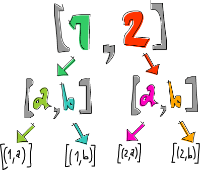
The list [1,2] gets bound to n and ['a','b'] gets bound to ch. Then, we do return (n,ch) (or [(n,ch)]), which means taking a pair of (n,ch) and putting it in a default minimal context. In this case, it's making the smallest possible list that still presents (n,ch) as the result and features as little non-determinism as possible. Its effect on the context is minimal. What we're saying here is this: for every element in [1,2], go over every element in ['a','b'] and produce a tuple of one element from each list.
Generally speaking, because return takes a value and wraps it in a minimal context, it doesn't have any extra effect (like failing in Maybe or resulting in more non-determinism for lists) but it does present something as its result.
Here's the previous expression rewritten in do notation:
listOfTuples :: [(Int,Char)]
listOfTuples = do
    n <- [1,2]
    ch <- ['a','b']
    return (n,ch)
This makes it a bit more obvious that n takes on every value from [1,2] and ch takes on every value from ['a','b']. Just like with Maybe, we're extracting the elements from the monadic values and treating them like normal values and >>= takes care of the context for us. The context in this case is non-determinism.
Using lists with do notation really reminds me of something we've seen before. Check out the following piece of code:
ghci> [ (n,ch) | n <- [1,2], ch <- ['a','b'] ]
[(1,'a'),(1,'b'),(2,'a'),(2,'b')]
Yes! List comprehensions! In our do notation example, n became every result from [1,2] and for every such result, ch was assigned a result from ['a','b'] and then the final line put (n,ch) into a default context (a singleton list) to present it as the result without introducing any additional non-determinism. In this list comprehension, the same thing happened, only we didn't have to write return at the end to present (n,ch) as the result because the output part of a list comprehension did that for us.
In fact, list comprehensions are just syntactic sugar for using lists as monads. In the end, list comprehensions and lists in do notation translate to using >>= to do computations that feature non-determinism.
List comprehensions allow us to filter our output. For instance, we can filter a list of numbers to search only for that numbers whose digits contain a 7:
ghci> [ x | x <- [1..50], '7' `elem` show x ]
[7,17,27,37,47]
We apply show to x to turn our number into a string and then we check if the character '7' is part of that string. Pretty clever. To see how filtering in list comprehensions translates to the list monad, we have to check out the guard function and the MonadPlus type class. The MonadPlus type class is for monads that can also act as monoids. Here's its definition:
class Monad m => MonadPlus m where
    mzero :: m a
    mplus :: m a -> m a -> m a
mzero is synonymous to mempty from the Monoid type class and mplus corresponds to mappend. Because lists are monoids as well as monads, they can be made an instance of this type class:
instance MonadPlus [] where
    mzero = []
    mplus = (++)
For lists mzero represents a non-deterministic computation that has no results at all — a failed computation. mplus joins two non-deterministic values into one. The guard function is defined like this:
guard :: (MonadPlus m) => Bool -> m ()
guard True = return ()
guard False = mzero
It takes a boolean value and if it's True, takes a () and puts it in a minimal default context that still succeeds. Otherwise, it makes a failed monadic value. Here it is in action:
ghci> guard (5 > 2) :: Maybe ()
Just ()
ghci> guard (1 > 2) :: Maybe ()
Nothing
ghci> guard (5 > 2) :: [()]
[()]
ghci> guard (1 > 2) :: [()]
[]
Looks interesting, but how is it useful? In the list monad, we use it to filter out non-deterministic computations. Observe:
ghci> [1..50] >>= (\x -> guard ('7' `elem` show x) >> return x)
[7,17,27,37,47]
The result here is the same as the result of our previous list comprehension. How does guard achieve this? Let's first see how guard functions in conjunction with >>:
ghci> guard (5 > 2) >> return "cool" :: [String]
["cool"]
ghci> guard (1 > 2) >> return "cool" :: [String]
[]
If guard succeeds, the result contained within it is an empty tuple. So then, we use >> to ignore that empty tuple and present something else as the result. However, if guard fails, then so will the return later on, because feeding an empty list to a function with >>= always results in an empty list. A guard basically says: if this boolean is False then produce a failure right here, otherwise make a successful value that has a dummy result of () inside it. All this does is to allow the computation to continue.
Here's the previous example rewritten in do notation:
sevensOnly :: [Int]
sevensOnly = do
    x <- [1..50]
    guard ('7' `elem` show x)
    return x
Had we forgotten to present x as the final result by using return, the resulting list would just be a list of empty tuples. Here's this again in the form of a list comprehension:
ghci> [ x | x <- [1..50], '7' `elem` show x ]
[7,17,27,37,47]
So filtering in list comprehensions is the same as using guard.
A knight's quest
Here's a problem that really lends itself to being solved with non-determinism. Say you have a chess board and only one knight piece on it. We want to find out if the knight can reach a certain position in three moves. We'll just use a pair of numbers to represent the knight's position on the chess board. The first number will determine the column he's in and the second number will determine the row.
Let's make a type synonym for the knight's current position on the chess board:
type KnightPos = (Int,Int)
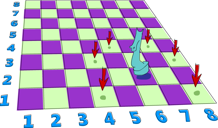
So let's say that the knight starts at (6,2). Can he get to (6,1) in exactly three moves? Let's see. If we start off at (6,2) what's the best move to make next? I know, how about all of them! We have non-determinism at our disposal, so instead of picking one move, let's just pick all of them at once. Here's a function that takes the knight's position and returns all of its next moves:
moveKnight :: KnightPos -> [KnightPos]
moveKnight (c,r) = do
    (c',r') <- [(c+2,r-1),(c+2,r+1),(c-2,r-1),(c-2,r+1)
               ,(c+1,r-2),(c+1,r+2),(c-1,r-2),(c-1,r+2)
               ]
    guard (c' `elem` [1..8] && r' `elem` [1..8])
    return (c',r')
The knight can always take one step horizontally or vertically and two steps horizontally or vertically but its movement has to be both horizontal and vertical. (c',r') takes on every value from the list of movements and then guard makes sure that the new move, (c',r') is still on the board. If it it's not, it produces an empty list, which causes a failure and return (c',r') isn't carried out for that position.
This function can also be written without the use of lists as a monad, but we did it here just for kicks. Here is the same function done with filter:
moveKnight :: KnightPos -> [KnightPos]
moveKnight (c,r) = filter onBoard
    [(c+2,r-1),(c+2,r+1),(c-2,r-1),(c-2,r+1)
    ,(c+1,r-2),(c+1,r+2),(c-1,r-2),(c-1,r+2)
    ]
    where onBoard (c,r) = c `elem` [1..8] && r `elem` [1..8]
Both of these do the same thing, so pick one that you think looks nicer. Let's give it a whirl:
ghci> moveKnight (6,2)
[(8,1),(8,3),(4,1),(4,3),(7,4),(5,4)]
ghci> moveKnight (8,1)
[(6,2),(7,3)]
Works like a charm! We take one position and we just carry out all the possible moves at once, so to speak. So now that we have a non-deterministic next position, we just use >>= to feed it to moveKnight. Here's a function that takes a position and returns all the positions that you can reach from it in three moves:
in3 :: KnightPos -> [KnightPos]
in3 start = do
    first <- moveKnight start
    second <- moveKnight first
    moveKnight second
If you pass it (6,2), the resulting list is quite big, because if there are several ways to reach some position in three moves, it crops up in the list several times. The above without do notation:
in3 start = return start >>= moveKnight >>= moveKnight >>= moveKnight
Using >>= once gives us all possible moves from the start and then when we use >>= the second time, for every possible first move, every possible next move is computed, and the same goes for the last move.
Putting a value in a default context by applying return to it and then feeding it to a function with >>= is the same as just normally applying the function to that value, but we did it here anyway for style.
Now, let's make a function that takes two positions and tells us if you can get from one to the other in exactly three steps:
canReachIn3 :: KnightPos -> KnightPos -> Bool
canReachIn3 start end = end `elem` in3 start
We generate all the possible positions in three steps and then we see if the position we're looking for is among them. So let's see if we can get from (6,2) to (6,1) in three moves:
ghci> (6,2) `canReachIn3` (6,1)
True
Yes! How about from (6,2) to (7,3)?
ghci> (6,2) `canReachIn3` (7,3)
False
No! As an exercise, you can change this function so that when you can reach one position from the other, it tells you which moves to take. Later on, we'll see how to modify this function so that we also pass it the number of moves to take instead of that number being hardcoded like it is now.
Monad laws

Just like applicative functors, and functors before them, monads come with a few laws that all monad instances must abide by. Just because something is made an instance of the Monad type class doesn't mean that it's a monad, it just means that it was made an instance of a type class. For a type to truly be a monad, the monad laws must hold for that type. These laws allow us to make reasonable assumptions about the type and its behavior.
Haskell allows any type to be an instance of any type class as long as the types check out. It can't check if the monad laws hold for a type though, so if we're making a new instance of the Monad type class, we have to be reasonably sure that all is well with the monad laws for that type. We can rely on the types that come with the standard library to satisfy the laws, but later when we go about making our own monads, we're going to have to manually check the if the laws hold. But don't worry, they're not complicated.
Left identity
The first monad law states that if we take a value, put it in a default context with return and then feed it to a function by using >>=, it's the same as just taking the value and applying the function to it. To put it formally:
- return x >>= f is the same damn thing as f x
If you look at monadic values as values with a context and return as taking a value and putting it in a default minimal context that still presents that value as its result, it makes sense, because if that context is really minimal, feeding this monadic value to a function shouldn't be much different than just applying the function to the normal value, and indeed it isn't different at all.
For the Maybe monad return is defined as Just. The Maybe monad is all about possible failure, and if we have a value and want to put it in such a context, it makes sense that we treat it as a successful computation because, well, we know what the value is. Here's some return usage with Maybe:
ghci> return 3 >>= (\x -> Just (x+100000))
Just 100003
ghci> (\x -> Just (x+100000)) 3
Just 100003
For the list monad return puts something in a singleton list. The >>= implementation for lists goes over all the values in the list and applies the function to them, but since there's only one value in a singleton list, it's the same as applying the function to that value:
ghci> return "WoM" >>= (\x -> [x,x,x])
["WoM","WoM","WoM"]
ghci> (\x -> [x,x,x]) "WoM"
["WoM","WoM","WoM"]
We said that for IO, using return makes an I/O action that has no side-effects but just presents a value as its result. So it makes sense that this law holds for IO as well.
Right identity
The second law states that if we have a monadic value and we use >>= to feed it to return, the result is our original monadic value. Formally:
- m >>= return is no different than just m
This one might be a bit less obvious than the first one, but let's take a look at why it should hold. When we feed monadic values to functions by using >>=, those functions take normal values and return monadic ones. return is also one such function, if you consider its type. Like we said, return puts a value in a minimal context that still presents that value as its result. This means that, for instance, for Maybe, it doesn't introduce any failure and for lists, it doesn't introduce any extra non-determinism. Here's a test run for a few monads:
ghci> Just "move on up" >>= (\x -> return x)
Just "move on up"
ghci> [1,2,3,4] >>= (\x -> return x)
[1,2,3,4]
ghci> putStrLn "Wah!" >>= (\x -> return x)
Wah!
If we take a closer look at the list example, the implementation for >>= is:
xs >>= f = concat (map f xs)
So when we feed [1,2,3,4] to return, first return gets mapped over [1,2,3,4], resulting in [[1],[2],[3],[4]] and then this gets concatenated and we have our original list.
Left identity and right identity are basically laws that describe how return should behave. It's an important function for making normal values into monadic ones and it wouldn't be good if the monadic value that it produced did a lot of other stuff.
Associativity
The final monad law says that when we have a chain of monadic function applications with >>=, it shouldn't matter how they're nested. Formally written:
- Doing (m >>= f) >>= g is just like doing m >>= (\x -> f x >>= g)
Hmmm, now what's going on here? We have one monadic value, m and two monadic functions f and g. When we're doing (m >>= f) >>= g, we're feeding m to f, which results in a monadic value. Then, we feed that monadic value to g. In the expression m >>= (\x -> f x >>= g), we take a monadic value and we feed it to a function that feeds the result of f x to g. It's not easy to see how those two are equal, so let's take a look at an example that makes this equality a bit clearer.
Remember when we had our tightrope walker Pierre walk a rope while birds landed on his balancing pole? To simulate birds landing on his balancing pole, we made a chain of several functions that might produce failure:
ghci> return (0,0) >>= landRight 2 >>= landLeft 2 >>= landRight 2
Just (2,4)
We started with Just (0,0) and then bound that value to the next monadic function, landRight 2. The result of that was another monadic value which got bound into the next monadic function, and so on. If we were to explicitly parenthesize this, we'd write:
ghci> ((return (0,0) >>= landRight 2) >>= landLeft 2) >>= landRight 2
Just (2,4)
But we can also write the routine like this:
return (0,0) >>= (\x ->
landRight 2 x >>= (\y ->
landLeft 2 y >>= (\z ->
landRight 2 z)))
return (0,0) is the same as Just (0,0) and when we feed it to the lambda, the x becomes (0,0). landRight takes a number of birds and a pole (a tuple of numbers) and that's what it gets passed. This results in a Just (0,2) and when we feed this to the next lambda, y is (0,2). This goes on until the final bird landing produces a Just (2,4), which is indeed the result of the whole expression.
So it doesn't matter how you nest feeding values to monadic functions, what matters is their meaning. Here's another way to look at this law: consider composing two functions, f and g. Composing two functions is implemented like so:
(.) :: (b -> c) -> (a -> b) -> (a -> c)
f . g = (\x -> f (g x))
If the type of g is a -> b and the type of f is b -> c, we arrange them into a new function which has a type of a -> c, so that its parameter is passed between those functions. Now what if those two functions were monadic, that is, what if the values they returned were monadic values? If we had a function of type a -> m b, we couldn't just pass its result to a function of type b -> m c, because that function accepts a normal b, not a monadic one. We could however, use >>= to make that happen. So by using >>=, we can compose two monadic functions:
(<=<) :: (Monad m) => (b -> m c) -> (a -> m b) -> (a -> m c)
f <=< g = (\x -> g x >>= f)
So now we can compose two monadic functions:
ghci> let f x = [x,-x]
ghci> let g x = [x*3,x*2]
ghci> let h = f <=< g
ghci> h 3
[9,-9,6,-6]
Cool. So what does that have to do with the associativity law? Well, when we look at the law as a law of compositions, it states that f <=< (g <=< h) should be the same as (f <=< g) <=< h. This is just another way of saying that for monads, the nesting of operations shouldn't matter.
If we translate the first two laws to use <=<, then the left identity law states that for every monadic function f, f <=< return is the same as writing just f and the right identity law says that return <=< f is also no different from f.
This is very similar to how if f is a normal function, (f . g) . h is the same as f . (g . h), f . id is always the same as f and id . f is also just f.
In this chapter, we took a look at the basics of monads and learned how the Maybe monad and the list monad work. In the next chapter, we'll take a look at a whole bunch of other cool monads and we'll also learn how to make our own.